HM Medical Clinic

Usgs open-file report 2005-1339

In Cooperation with the Southern Nevada Water Authority
Gravity Studies of Cave, Dry Lake, and Delamar
Valleys, East-Central Nevada
By Daniel S. Scheirer Any use of trade, firm, or product names is for descriptive purposes only and does not imply endorsement by the U.S. Government Open-File Report 2005-1339 U.S. Department of the Interior
U.S. Geological Survey

Contents
Gravity Studies of Cave, Dry Lake, and Delamar
Valleys, East-Central Nevada
By Daniel S. Scheirer Abstract
Analysis of gravity anomalies in Cave, Dry Lake, and Delamar valleys in east-central Nevada defines the overall shape of their basins, provides estimates of the depth to pre-Cenozoic basement rocks, and identifies buried faults beneath the sedimentary cover. In all cases, the basins are asymmetric in their cross section and in their placement beneath the valley, reflecting the extensional tectonism that initiated during Miocene time in this area. Absolute values of basin depths are estimated using a density-depth profile calibrated by deep oil and gas wells that encountered basement rocks in Cave Valley. The basin beneath southern Cave Valley extends down to 6.0 km, that of Dry Lake Valley extends to 8.2 km, and that of Delamar Valley extends to 6.4 km. The ranges surrounding Dry Lake and Delamar valleys are dominated by volcanic units that may produce lower-density basin infill, which in turn, would make the maximum depth estimates somewhat less. Dry Lake Valley is characterized by a slot-like graben in its center, whereas the deep portions of Cave and Delamar valleys are more bowl-shaped. Significant portions of the basins are shallow (<1 km deep), as are the transitions between each of these valleys. A seismic reflection image across southern Cave and Muleshoe valleys confirms the basin shapes inferred from gravity analysis. The architecture of these basins inferred from gravity will aid in interpreting the hydrogeologic framework of Cave, Dry Lake, and Delamar valleys by placing estimates on the volume and connectivity of potential unconsolidated alluvial aquifers and by identifying faults buried beneath basin deposits. In the southern half of Nevada, ground water is organized into a number of extensive regional flow systems (e.g., Harrill and Prudic, 1998) where ground water can flow between adjacent topographic ranges and basins. Subsurface flow occurs within permeable units or along permeable geologic structures. In east-central Nevada, the main flow system is the White River regional ground water flow system (e.g. Eakin, 1966), or alternatively termed the Colorado regional flow system (Harrill and Prudic, 1998). Aquifer units include widely distributed Paleozoic carbonate rocks, locally significant Tertiary volcanic rocks, and Cenozoic basin-fill deposits (cf., Plume and Carlton, 1988, Dettinger and others, 1995, and Harrill and Prudic, 1998). Regional aquifer recharge in the White River flow system occurs by precipitation in primarily the northern mountainous areas with the primary discharge occurring at Muddy River Springs, which form the Muddy River (Dettinger and others, 1995; Page and others, in press). The valleys that are the focus of this study: Cave, Dry Lake, and Delamar, are situated near the center of the White River regional ground-water flow system, in Lincoln and White Pine counties (Figure 1). Precambrian crystalline basement does not crop out in this area, but is thought to form a deep barrier to ground water transport (D'Agnese and others, 1997). The ranges surrounding the study basins primarily consist of Paleozoic marine rocks, predominantly carbonate units but also minor shale, conglomerate, and quartzite rocks that formed on the western continental margin of North America, and of Tertiary volcanic rocks, Figure 1b (e.g., Tschanz and Pampeyan, 1970; Stewart, 1980). Marine deposition was nearly continuous in this area throughout the Paleozoic, and deposition ceased until continental volcanism, minor intrusion and plutonism, and associated sedimentation occurred during Oligocene and Miocene times. The Caliente caldera complex, in the southern portion of the study area, forms a thick and variable sequence of volcanics that comprise some of the ranges in the south (Figure 1b). Tectonism initiated in the study area in Miocene time and deformed the Paleozoic units and older volcanics via extensional block-faulting and subsidiary faulting, leading to the present-day basin and range landscape. Erosion of the ranges filled adjacent valleys with alluvial sequences that are unconsolidated or poorly consolidated, and basin-fill occupies about 50% of the exposure within the study area (Figure 1b). In the study area, the geological structures defining the northern ranges, Egan and Schell Creek, are simpler than their counterparts to the south. In the north, the units comprising the ranges dip primarily to the east with steep, range-front normal faults marking their western margins; in the south, the ranges are built of a combination of Paleozoic marine rocks and variably-thick Tertiary volcanic rocks, and they are disrupted by complex arrays of faults related both to the regional extension and to stresses from volcanic processes (Tschanz and Pampeyan, 1970). The U.S. Geological Survey conducted gravity experiments along Cave, Dry Lake, and Delamar valleys (Figure 1) to help delineate the subsurface configuration of the valleys and to identify faults that may lie beneath alluvial cover. Because of the substantial density contrast between unconsolidated sediments and older marine sedimentary rocks, gravity is a useful tool for this goal. Gravity Observations and Analysis
In 2003 and 2004, the U.S. Geological Survey collected gravity observations at 468 new sites (Appendix Table A1) to supplement the prior compilation of 3500 stations in this area (Snyder and others, 1981; Bol and others, 1983; Snyder and others, 1984; Ponce, 1992, 1997). For the recent fieldwork, we established local gravity base stations at the Lanes Ranch Motel, Lund, Nev., at the Hot Springs Motel, Caliente, Nev., and at the Union Pacific Train Station, Caliente, Nev. (Table 1). Values of gravity at these local bases were tied to the IGSN71 gravity datum (Morelli, 1974) via double-loop surveying to the ELYA benchmark at the Ely (Nev.) Airport. New data were collected with a LaCoste-Romberg gravity meter, and station positions were recorded with a Trimble GeoXT Global Positioning System (GPS) receiver. By using fixed GPS reference stations within 100 km of the gravity observations, latitude and longitude values were calculated via post-processing to have a precision generally better than 1 meter, and elevations had precisions of about 1 meter. At gravity stations situated on outcrop, we collected 153 rock hand-samples at 152 of the stations (Appendix Table A2), and we measured their density and magnetic susceptibility properties in the lab (Johnson and Olhoeft, 1984). Values of observed gravity were calculated at the new stations by accounting for fluctuations related to tidal accelerations and for instrument drift constrained at the beginning and end of each field day. New gravity stations were collected within coverage gaps of the prior data, especially in the ranges adjacent to the study basins. We used a helicopter to collect many of the stations in rugged terrain (138 sites). Characterizing the gravity variations within the ranges is required to allow accurate separation of the observed gravity anomalies into pre-Cenozoic and Cenozoic contributions, as described in the depth to basement technique below. For both the prior and new gravity stations, we compared measured station elevations to corresponding elevations of the 10 m (and 30 m in a few areas where higher resolution was unavailable) digital elevation models (DEMs). Where the station elevations differed by 80 feet (24.4 m) or more from the DEM, the gravity station was omitted from further analysis. Where the station elevations differed by a lesser but still significant amount, we inspected those cases and manually removed some of these stations, as well. We then calculated a series of predictable gravity corrections for all of the stations to account for: the global gravity field, the reduction in gravity with increasing elevation (free-air correction), the effect of mass between the station and the geoid (simple Bouguer correction), the effect of topographic variation near the station (terrain correction), and the effect of compensating mass near the base of the crust (isostatic correction). The final gravity anomaly after application of these corrections is termed the isostatic gravity anomaly and is useful for interpretation because it primarily reflects the density variations in the upper- and mid-crust (Simpson and others, 1986). For new gravity stations, estimates were made of the field terrain correction in a zone from the station out to a radius of 68 m; for the prior stations, this innermost terrain correction was not available. For all stations, digital terrain corrections beyond 68 m were calculated from DEMs in two stages: from 68 m to 2 km and from 2 km to 167 km using the algorithm of Plouff (1997). Other parameters that were used in the calculation of gravity corrections are typical for gravity studies in the Basin and Range Province; these include an upper crustal density of 2.67 g/cc, a mantle-crust density contrast of 0.4 g/cc, and a nominal crustal thickness at sea level of 25 km. A typical error of the new gravity stations is estimated to be 0.2 mGal, and a typical error of the prior gravity stations is thought to be 0.5-1 mGal. In all cases, the errors are primarily due to elevation and terrain correction uncertainties, and they are small relative to the size of the anomalies that arise from basin structures. Gravity station data were gridded with a 500 m spacing, which is somewhat finer than the average station- spacing in the valleys ( 1 km) and significantly finer that the spacing in the ranges, where gaps up to 4 km exist despite filling in many gaps via helicopter. During the gridding process, we identified a number of prior stations that had gravity values significantly different from their neighbors. To aid in identifying these noise spikes, we upward-continued (e.g., Blakely, 1996) the isostatic gravity field by 500 m, then calculated the difference between the original and upward-continued grids. This difference highlights short-wavelength anomalies in the grid, and individual gravity stations that contributed significant noise were identified and omitted from further analysis. Of the 3900 gravity stations in the study area, 67 were omitted because their station elevations differed significantly from the DEM values, and 9 of the remaining stations were omitted because of gravity noise spikes. All of the stations collected in 2003 and 2004 passed the noise-editing tests. Gridded isostatic gravity anomaly data were used to guide the gravity analysis in two modes: to detect significant lateral density interfaces in the subsurface using a maximum horizontal gradient technique (Blakely and Simpson, 1986) and to create models of the depth to pre-Cenozoic basement using the anomaly separation technique of Jachens and Moring (1990). Maximum horizontal gradients of gravity fields are situated above vertical or near-vertical density boundaries in the subsurface, especially for shallow sources. The positions of local maxima of the gravity gradient can help delineate lithologic contacts at depth, especially those related to faults juxtaposing low-density basin fill against consolidated rock. The magnitude of the gradient is a function of the depth to the density boundary and the size of the density contrast, and in practice, the presence of noise in the gravity grid may lead to false identifications of geological boundaries using this technique. The interpretive power of this method is best where maximum gradients are spatially identified in clusters or lineaments. The depth-to-basement technique endeavors (1) to separate contributions to the isostatic gravity anomaly that arise from Cenozoic sedimentary and volcanic deposits and those from pre-Cenozoic rocks and (2) to convert the low-density contributions from the young deposits into a model of basin depth (Jachens and Moring, 1990). This is an inverse geophysical approach because it calculates model geometry from observations of gravity, constrained by outcrop patterns and with a priori assumptions about the density contrast of basin fill relative to surrounding rocks. This method is iterative and has been successfully applied to the entire Basin and Range Province (Saltus and Jachens, 1995) and to individual basins and groups of basins in southern Nevada (e.g., Langenheim and others, 2000). The depth-to-basement method first separates those gravity stations that lie on Cenozoic deposits (termed "basin") vs. those that lie on pre-Cenozoic rocks; these older units are termed "basement" in this description, a usage that differs from the common description of old, crystalline rocks as basement in many areas. The isostatic gravity anomalies at basement stations are then interpolated across the intervening basins, and differences between the interpolated basement gravity values and those measured at basin stations are attributed to the low-density basin infill. Using a 1-D approximation, the depth of the basin fill is estimated from the size of the basin gravity anomaly at each grid point, and then the gravitational attraction of these interpreted basins is calculated. Where a basement gravity station lies close to basin material, some of the attraction of the low-density infill will influence its gravity value; thus, the calculated basin attraction must removed from the gravity value at each basement station. This process yields estimates of basement gravity, basin gravity, and depth to basement beneath the basins. This sequence is then repeated for multiple iterations until the estimates of basin depth converge. In this study, gravity stations are separated based on their placement on three geological units: pre-Cenozoic basement, Cenozoic sedimentary fill, and Cenozoic volcanic deposits. The depth of the resulting basement surface is assumed to be the thickness of sedimentary deposits where sediments are at the surface and to be the thickness of volcanic deposits where volcanics crop out, although it is likely that sediments overly volcanic deposits in some areas. A critical input to the depth-to-basement method is the depth variation of the density contrast of the basin fill material relative to the surrounding rock; this density profile is the link to convert basin gravity anomalies to basin depth estimates. Measured density-depth functions are available from deep boreholes in other parts of the Basin and Range Province (e.g. Healey and others, 1984) but not from the study area. We first utilized the density-depth functions used in Jachens and Moring (1990) that were deemed appropriate for the entire Basin and Range Province (Table 2). After some experimentation, discussed below, we adopted density-depth relationships (Table 2) with smaller density contrasts, leading to deeper estimated basins that matched better independent constraints on basement depths. In these density-depth functions, density increases with depth, especially within the uppermost 600 m. Near the surface, sedimentary deposits are less dense than the volcanics; deeper than 600 m, the density- depth functions are identical. This relationship demonstrates why it is very difficult to separate the geophysical effects of sedimentary and volcanic deposits using gravity methods. Measured depths to the base of Cenozoic deposits can be used as important constraints to the depth-to- basement estimation. These measurements are available typically from deep boreholes associated with oil and gas exploration (Table 3 indicates those available in Cave and Dry Lake valleys, Hess, 2004), and even if a borehole does not penetrate the entire basin deposit, its bottom depth may be used as a minimum constraint on the depth-to-basement solution. In this area, four deep wells from the MX project (Bunch and Harrill, 1984) are also available for comparison with gravity models (Table 3). Independent basement depth constraints may be applied to the modeling using two approaches: either as a priori exact and minimum depth constraints that must be satisfied as the depth-to-basement algorithm iterates, or as post-modeling validation of the depth-to-basement solution. Deciding on which approach to use depends on the distribution of depth constraints and on the availability of measured density-depth functions in the study area. The latter post-modeling approach is utilized in this study for two reasons: deep borehole constraints are sparse, and systematic differences in measured basin depths (from boreholes) and estimated depths (from gravity analysis) will allow testing and modification of the assumed density-depth function. As noted above and described below, we modified the density-depth function of Jachens and Moring (1990) to match borehole depths in Cave Valley more closely. Rock property measurements are summarized in Table 4 as averages grouped by rock type. While physical properties of individual hand-samples may not represent well the bulk properties of in situ volumes of rock, especially those at depth, the measurements can aid in establishing the density variations among the units. The most common rock types sampled, carbonate and felsic volcanic rocks, have statistically distinct average densities of 2.70 g/cm3 and 2.34 g/cm3, respectively. The Paleozoic rock samples, as a whole, average to a density value very close to the 2.67 g/cm3 assumed for the Bouguer and isostatic gravity corrections. The young volcanic rocks are less dense and more porous (2-10%) than the older sedimentary rocks (<3% porosity). The volcanic rocks are also the only samples to have significantly non-zero magnetic susceptibility. The results of the gravity analysis are presented as a series of maps in Figure 2 for Cave and northernmost Dry Lake valleys (including Muleshoe Valley) and in Figure 3 for Dry Lake and Delamar valleys. Cave Valley is bounded by the sinuous Egan and Schell Creek ranges and is segmented into northern and southern halves by the Shingle Pass Fault that bends the southern Egan Range towards the northeast and across much of the oval-shaped valley floor (Figure 2b, Tschanz and Pampeyan, 1970). These ranges are primarily eastward-dipping tilt-blocks with steep normal faults defining their western margins. Smaller faults cross the ranges, segment the ranges into distinct sections, and create topographic passes. Volcanic units are present in a number of areas surrounding Cave Valley but not with significant thickness (Tschanz and Pampeyan, 1970). The southern portion of Cave Valley has a playa and is much flatter than the floor of the northern valley, which is dissected by streams and is marked by a handful of isolated outcrops (Figure 2b). For Cave Valley, the prior gravity station distribution was adequate for much of the valley area, but there were large gaps in the surrounding Egan and Schell Creek ranges that were filled using helicopter access (Figure 2a). Many of the gaps that remain within the ranges were investigated by air but deemed unsafe as landing sites. Numerous stations in the valley floors were collected to fill existing gaps, to survey along the ECN-01 seismic line, and to collect gravity observations at well sites that provide independent information on depth to the base of valley-fill deposits. In Cave Valley proper, there are 8 oil and gas wells that penetrated basement, and 1 MX well that encountered basement (Figure 2a and Table 3). The isostatic gravity anomaly of Cave and Muleshoe valleys is characterized by 20-30 mGal lows centered on the valleys relative to the isostatic values in the surrounding ranges. There are significant gravity fluctuations within the ranges, reflecting the lithologic variation within them; for example, the low-relief range along the southeastern margin of Muleshoe Valley is comprised of volcanic rocks and has a relative gravity low (Figures 2b, 2c). The maximum horizontal gradients of the isostatic anomaly over areas with surface sediments are displayed as pink symbols on the isostatic gravity map (Figure 2c). Larger and more continuous maximum gradient picks are present in southern Cave Valley relative to northern Cave Valley. In the south, two main lines of maximum gradients are found paralleling the eastern and western margins of the valley, with the western group close to the axis of the valley and the eastern group close to the front of the Schell Creek Range. Muleshoe Valley is also lined by steep isostatic gravity gradients along its eastern and western margins, and is marked by diffuse and small gradients on its southern margin where it crosses a small rise that leads into northernmost Dry Lake Valley (Figure 2a, 2c). The depth-to-basement algorithm separates the isostatic gravity anomaly into portions that arise from the Cenozoic deposits ("basin-fill") vs. those from the pre-Cenozoic rocks ("basement"), and the resulting basin gravity anomaly is illustrated in Figure 2d. The basin gravity anomaly is zero or slightly negative for areas of pre-Cenozoic outcrop, and it achieves the most negative values towards the centers of basins. This anomaly is transformed, via the assumed density-depth function, into a basement depth map, Figure 2e. Basin depths estimated from gravity extend to 6.0 km in Cave Valley. Maximum depth estimates from the adjacent valleys to the west (White River) and to the east (Lake) are greater, but the gravity coverage is not complete in these areas and careful calibration with independent basement depth constraints has not been performed. In northern Cave Valley, typical basement depths are hundreds of meters, and no site has an estimated depth greater than 1 km. Isolated outcrops extending to the northeast of the Shingle Pass Fault are surrounded by sediments no thicker than 100 m, based on this gravity analysis (Figure 2e). In southern Cave Valley, the basin has depth-to-basement estimates >1 km for more than half of its length; its deepest inferred depth is just east of the valley's axis. The borehole picks to the base of the alluvium are superimposed on the depth-to-basement map (Figure 2e) and show broad agreement in map-view. For comparison, the depth-to-basement map for this area from Saltus and Jachens (1995) is illustrated in Figure 2f. The most striking difference between these two solutions is the 4-fold (500 m vs. 2000 m) resolution increase of the new analysis and its attendant ability to characterize better the geological structures, such as range-front faults, in the study valleys. In addition, the depths of the new estimates are nearly 50% deeper because of the improved density-depth functions (Table 2). The results of comparisons between the base of alluvium picks from oil and gas wells (Hess, 2004) and MX wells (Table 3) and the depth-to-basement values from the gravity inversion are illustrated in Figure 4. Over the 0 to 2000 m depth range of basement identifications from wells, the estimated basement depths from gravity are centered about the 1:1 equivalence line. Using the greater density-contrast profiles of Jachens and Moring (1990) yielded results where the deeper wells significantly and systematically underestimated the measured basement depths. The match between measured and estimated basement depths is not perfect, and this might stem from a number of reasons: the downhole basement identification might be in error, the identification for a single borehole might not be representative of the true interface at depth averaged over the lateral dimension that contributes to the gravity anomaly measured at the earth's surface, errors in observed or reduced gravity will translate into errors in inferred depth, and densities in the basin deposits likely vary from place to place. While there is some scatter, the overall consistency between the basement depth estimates in this study indicate that the overall form of the depth-to-basement inversions are as correct as can be achieved with the available subsurface observations. It is important to note that observed borehole depths in Cave Valley extend to at most 1900 m, so we cannot test the density-contrast function values between that depth and depths more than twice as great. The two minimum depth constraints, gray circles in Figure 4, should fall to above the 1:1 equivalence line; these wells are located in Dry Lake and Delamar valleys and are discussed below. 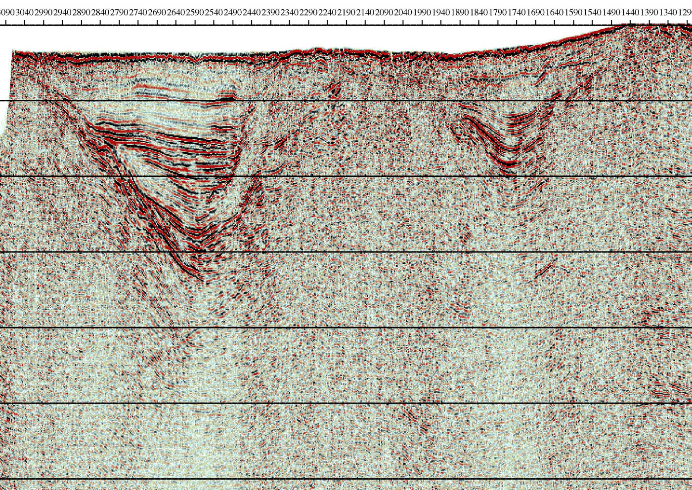An additional view into the subsurface structure of southern Cave Valley and Muleshoe valley is provided by a portion of the industry-shot ECN-01 seismic reflection line (Figure 5). The seismic line crosses near the maximum depth position of Cave Valley (Figure 2e). The seismic reflection image illustrates the asymmetric character of Cave Valley cross section, with a steeper eastern side where the range-front fault of the Schell Creek Range lies and a less-steep western floor leading up to the dip-slope of the Egan Range (Figure 5a). Strong reflectors mark the base of Cave Valley, and a discordant and more horizontal packet of reflectors characterizes much of the deeper valley fill. Weaker subhorizontal reflectors are present in the upper valley fill. The reflectors in the shallow portions of Muleshoe Valley are weak or absent, but in its deeper section exhibit characteristics similar to those of the Cave Valley reflectors. These seismic data are displayed in travel-time, so a quantitative appraisal of seismic depths to basement is not possible. Nevertheless, the inferred basin structure from gravity analysis (Figure 5b) shares a number of similarities with the seismic image: Cave Valley is asymmetric and reminiscent of a half-graben and the overall shapes of Cave vs. Muleshoe, in deeper portions, look similar between the seismic and gravity models. American Petroleum Institute (API) well 27-017-05221 is superimposed schematically on Figure 5b to illustrate its general agreement with the gravity depth-to-basement estimate and to show its position with respect to the seismic structures. Dry Lake Valley is bounded by the North Pahroc Range in the west and the Highland and Bristol ranges in the east, and the valley is marked by low saddles to the north and south. The surrounding ranges are intensely faulted and are comprised more of volcanic units than are the ranges surrounding Cave Valley (Tschanz and Pampeyan, 1970). Stations were added throughout the valley and adjacent ranges (Figure 3a). The isostatic gravity anomaly has a >30 mGal negative value in the center of the valley; large maximum horizontal gradients mark an area slightly displaced to the east of the valley axis, and smaller gradients delineate the ends of the basin (Figure 3c). The basin gravity anomaly (Figure 3d) emphasizes the narrowness of the central basin gravity anomaly, which has an aspect ratio of 5 and a magnitude 10 mGal greater than the anomaly in Cave Valley. The depth-to-basement solution for Dry Lake Valley exhibits a narrow slot-like depression along most of the valley that is slightly displaced to the east of the valley's centerline. Away from the slot, basin depths are generally <1 km, and within the slot most depths are >3 km and some are as deep as 8 km. No deep oil and gas or MX wells provide independent measures of basin depth in Dry Lake Valley, so the accuracy of the gravity to depth conversion depends on the appropriateness of the assumed density-depth function utilized in this study (Table 2) that was constrained in Cave Valley. Because the ranges surrounding Dry Lake Valley are composed predominantly of Tertiary volcanics, the sedimentary infill might have lower density than in Cave Valley, in which case the density contrasts with bedrock would be larger and the inverted basin depths would be shallower. Using the density-depth function of Jachens and Moring (1990), Dry Lake Valley would have a maximum basin depth of 6 km. Notwithstanding the question of the magnitude of the basin floor topography, the shape of the basin slot, with relatively flat shelves leading to the adjacent ranges, is robust and independent of any particular density-depth assumptions. No seismic lines are available across Dry Lake Valley, so models of the basin geometry depend on the analysis and interpretation of gravity data alone. Delamar Valley (Figure 3) is surrounded by volcanic ranges to the west, south, and east that are highly faulted. The isostatic gravity anomaly is similar to those in the other valleys in the study area, but the maximum horizontal gradients are only sporadically clustered along some sections of the South Pahroc (to the west) and Delamar (to the east) ranges. These ranges have lower isostatic gravity anomalies relative to ranges comprised of older, non-volcanic rocks, illustrating their low average densities (Figure 3c), despite the presence of shallow and dense Proterozoic rocks at the Delamar mining district to the east of the valley. The basin gravity anomaly (Figure 3d) has a minimum restricted to the southern half of Delamar Valley, which leads to the bowl-shaped basin inferred from the gravity inversion (Figure 3e). The maximum depth is almost 6.5 km, and it is located west of the center of the southern portion of Delamar Valley. Elsewhere, much of the valley has depths of 1-2 km. Again, no exact constraints on basement depth are available from well picks, so the inferred depths are based on calibration at Cave Valley. Like Dry Lake Valley, the volcanic ranges surrounding Delamar Valley likely create lower-density basin infill than in Cave Valley, where the density-depth profile was validated. Assuming the Jachens and Moring (1990) density function that utilizes lower-densities that used in this study, the deepest part of Delamar Valley would be 4 km below the valley floor. Discussion
The basin shapes of Cave, Dry Lake, and Delamar valleys are well discerned by gravity analysis, and they have distinct characters. The northern Cave Valley basin is filled by a thin (<1 km) accumulation of sediments that is discontinuous, except for a <100 m layer, with the deeper southern Cave Valley basin. The deeper basin has the form of an elongate bowl, with asymmetric sides that reflect the block faulting of the Egan and Schell Creek ranges. Muleshoe Valley is a shallower basin that is more symmetric than Cave Valley. In Dry Lake Valley, the deep basin is a narrow slot within the interior of the valley and running along most of its length. While the surrounding ranges are highly tectonized, the most significant faults buried beneath the sedimentary deposits are displaced away from the range fronts to form a slot-like graben in Dry Lake Valley. Whether the shoulders to the graben are simply buried, erosional pediment surfaces or whether they are regions between distinct fault systems proximal and distal to the range-fronts is unknown without further geological and geophysical observations. The southern portion of Delamar Valley is bowl-shaped and significantly deeper than the northern half of the valley. A small, 1-km deep basin-divide between the Delamar and Dry Lake valley basins occurs 5 km north of the subtle topographic divide between the valleys. One common feature of all of the study basins is that their maximal depths occur where the valley elevations are lowest, indicating a long-term connection between the geologic structures that deepen the basins and those that govern geomorphology in the study area. In Cave, Dry Lake, and Delamar Valleys, the size and shape of the surface playas are good proxies for the locations of maximal basin depths. Uncertainty in the density-depth profiles utilized in the depth-to-basement process translates into the greatest uncertainties in magnitude of basin depths. For Cave Valley, the oil and gas wells that penetrate basin infill to depths 35% of the maximum modeled depths are useful to constrain the density-depth function at shallow levels. Performing velocity analysis and depth migration of the ECN-01 seismic reflection line would add another independent constraint of the deep basin depths across southern Cave Valley, but the accuracy of these depths would depend on the quality of the velocities recovered from the seismic records. In the Dry Lake and Delamar valleys, neither deep borehole nor seismic constraints are available, so the actual basin depths could vary from those shown in this study. If the material filling the southern valleys is dominated by lower density volcanic units than the dominant Paleozoic rocks of Cave Valley, then the basin-fill density contrasts in Dry Lake and Delamar valleys are likely to be greater, which would lead to shallower basement surfaces inferred from gravity analysis in these southern basins. The trade-off between the assumed physical properties of the basin material and the magnitude of the resultant depth solutions is a fundamental limitation of interpreting potential fields, such as gravity. Analysis of gravity anomaly gradients indicates that buried faults generally bound the deepest portions of basins and that these faults are continuous and steep over much of the length of the basins. There is no clear association of inferred buried faults and those that criss-cross the surrounding ranges, indicating that if the exposed faults continue beneath the basin infill, they do not juxtapose units of significant density contrast nor do they play a major role in defining the gross architecture of the basin. The basin architecture inferred from gravity analysis will aid in interpreting the hydrogeologic framework of Cave, Dry Lake, and Delamar valleys in a number of ways. First, the depth-to-basement analysis allows estimation of the placement and volumes of basin-fill aquifers and their potential connections between basins. As noted above, most of the basins are asymmetric in shape and position within a valley, and they have only shallow connections from one basin to another. Second, buried valley-parallel faults are continuous along all of the basins, but these occur in different positions with respect to the valley center and range-fronts. The faults within Dry Lake Valley form a slot-like graben that is distinct from the bowl-shaped basins of southern Cave and Delamar valleys. Other geophysical or geological observations are required to assess how continuous these faults are beneath the basin fill, continuity that would have significant implications for ground-water connections in the carbonate aquifer system. We thank the Southern Nevada Water Authority for project funding. We are grateful to Robert Morin, Bruce Chuchel, and Allegra Hosford Scheirer for their assistance in the field, to Jeremy Lui for lab assistance, and to John Miller who processed the ECN-01 seismic data. This study was improved by reviews of Gary Dixon, Thomas Hildenbrand, Edward Mankinen, and David Ponce. Table 1. Gravity base stations used for data collected in 2003 and 2004. [Datums: latitude and longitude, NAD27; elevations, NGVD29; gravity values, IGSN71] Base name
Latitude
Longitude
Elevation (m)
Observed gravity
Description
Ely Airport, Nev. Lanes Ranch Motel, Union Pacific Stn., 1Part of the World Reference Gravity Network (Jablonsky, 1974) Table 2. Cenozoic density-depth functions. [Density contrasts are basin infill-density minus surrounding bedrock density] Depth range (km)
Sedimentary density
Volcanic density
Sedimentary density
Volcanic density
contrast (g/cm3)
contrast (g/cm3)
contrast (g/cm3)
contrast (g/cm3)
(Jachens & Moring, 1990)
(Jachens & Moring, 1990)
(this study)
(this study)
0-0.2 -0.65 -0.45 0.2-0.6 -0.55 -0.40 -0.50 0.6-1.2 -0.35 -0.35 -0.30 >1.2 -0.25 -0.25 Table 3. Deep borehole basement constraints. [Datums: latitude and longitude, NAD27; elevations, NGVD29] Well ID1 Valley
Latitude
Longitude
elevation
Total depth
Depth to basement
37° 26.65'N 114° 1API number for oil and gas wells; valley name for MX wells. Table 4. Average physical properties of rock samples, grouped by rock type. [Average property values are followed by 1-standard deviation values in parentheses.] Rock type
Number of
Grain density
Saturated bulk
Dry bulk density
Porosity
density (g/cm3)
(10-3 SI)
Interm. Volcanic Literature Cited
Blakely, R.J., 1996, Potential Theory in Gravity and Magnetic Applications: Cambridge University Press, 441 p. Blakely, R.J., and Simpson, R.W., 1986, Approximating edges of source bodies from magnetic or gravity anomalies: Geophysics, v. 51, p. 1494-1498. Bol, A.J., Snyder, D.B., Healey, D.L., and Saltus, R.W., 1983, Principal facts, accuracies, sources, and base station descriptions for 3672 gravity stations in the Lund and Tonopah 10 x 20 quadrangles, Nevada: available from National Technical Information Service, U.S. Department of Commerce, Springfield, VA 22152, PB81-1780, 86 p. Bunch, R.L., and Harrill, J.R., 1984, Compilation of selected hydrologic data from the MX missile-siting investigation, east-central Nevada and western Utah: U.S. Geological Survey Open-File Report 84-702, 123 p. D'Agnese, F.A., Faunt, C.C., Turner, K., and Hill, M.C., 1997, Hydrogeologic evaluation and numerical simulation of Death Valley regional ground-water flow system, Nevada and California: Water Resources Investigations Report 96-4300, 124 p. Dettinger, M.D., Harrill, J.R., Schmidt, D.L, and Hess, J.W., 1995, Distribution of carbonate-rock aquifers and the potential for their development, southern Nevada and adjacent parts of California, Arizona, and Utah: U.S. Geological Survey Water Resources Investigations Report 91-4146, 100 p. Eakin, T.E., 1966, A regional interbasin groundwater system in the White River area, southeastern Nevada: Water Resources Research, v. 2, p. 251-271. Harrill, J.R., and Pruric, D.E., 1998, Aquifer systems in the Great Basin region of Nevada, Utah and adjacent sates – Summary report: U.S. Geological Survey Professional Paper 1409A, 61p. Healey, D.L, Clutsom, F.G., and Glover, D.A., 1984, Borehole gravity meter surveys in drill holes USW G-3, UE-25p1, and UE-25c1: U.S. Geological Survey Open-File Report 84-672, 16 p. Hess, R.H., 2004, Nevada oil and gas well database (NVOILWEL), Nevada Bureau of Mines and Geology Open-File Report 04-1, Jablonski, H. M., 1974, World relative gravity reference network North America, Parts 1 and 2: U.S. Defense Mapping Agency Aerospace Center Reference Publication no. 25, originally published 1970, revised 1974, with supplement of IGSN 71 gravity datum values, 1261 p. Jachens, R.C., and Moring, B.C., 1990, Maps of the thickness of Cenozoic deposits and the isostatic residual gravity over basement for Nevada: U.S. Geological Survey Open-File Report 90-404, 15 p., 2 plates, scale 1:1,000,000. Johnson, G.R., and Olhoeft, G.R., 1984, Density of rocks and minerals, in Carmichael, R.S., ed., CRC Handbook of Physical Properties of Rocks, Vol. 3: Boca Raton, Fla., CRC Press, Inc., p. 1-38. Langenheim, V.E., Glen, J.M., Jachens, R.C., Dixon, G.L., Katzer, T.C., and Morin, R.L., 2000, Geophysical constraints on the Virgin River depression, Nevada, Utah, and Arizona: U.S. Geological Survey Open-File Report 00-407, 26 p. Morelli, C., 1974, The International Gravity Standardization Net 1971: International Association of Geodesy Special Publication no. Page, W.R., Dixon, G.L., Rowley, P.D., and Brickey, D.W., in press, Geologic map of the White River flow system and adjacent areas, Nevada, Utah, and Arizona: Nevada Bureau of Mines and Geology Map Series, 1:250,000 scale. Plouff, D., 1977, Preliminary documentation for a FORTRAN program to computer gravity terrain corrections based on topography digitized on a geographic grid: U.S. Geological Survey Open-File Report 77-535, 45 p. Plume, R.W., and Carlton, S.M., 1988, Hydrogeology of the Great Basin region of Nevada, Utah, and adjacent states: U.S. Geological Survey Hydrologic Investigations Atlas HA-694-A, scale 1:1,000,000. Ponce, D.A., 1992, Bouguer gravity map of Nevada – Ely sheet: Nevada Bureau of Mines and Geology Map 99, scale 1:250,000. Ponce, D.A., 1997, Gravity data of Nevada: U.S. Geological Survey Digital Data Series DDS-42, 27 p, CD-ROM. Saltus, R.W., and Jachens, R.C., 1995, Gravity and basin-depth maps of the Basin and Range Province, western United States: U.S. Geological Survey Geophysical Investigations Map GP-1012, 15 p., scale 1:2,500,000. Simpson, R.W., Jachens, R.C., Blakely, R.J., and Saltus, R.W., 1986, A new isostatic residual gravity map of the conterminous United States with a discussion on the significance of isostatic residual anomalies: Journal of Geophysical Research, v. 91, p. 8348-8372. Snyder, D.B., Wahl, R.R., and Currey, F.E., 1981, Bouguer gravity map of Nevada – Caliente sheet: Nevada Bureau of Mines and Geology Map 70, scale 1:250,000. Snyder, D.B., Healey, D.L., and Saltus, R.W., 1984, Bouguer gravity map of Nevada – Lund sheet: Nevada Bureau of Mines and Geology Map 80, scale 1:250,000. Stewart, J.H., 1980, Geology of Nevada: Nevada Bureau of Mines and Geology Special Publication 4, 136 p. Stewart, J.H., and Carlson, J.E., 1978, Geologic map of Nevada: U.S. Geological Survey, scale 1:500,000. Tschanz, C.M., and Pampeyan, E.H., 1970, Geology and mineral deposits of Lincoln County, Nevada: Nevada Bureau of Mines and Geology Bulletin 73, 188 p.

ch John Mtn. 38˚30'
uleshoe ist
Grouped Geologic Units (Stewart and Carlson, 1978) Cenozoic sediments Pre-Cenozoic sedimentary Felsic volcanic rocks Felsic intrusive rocks Mafic volcanic rocks 2000 4000 6000 8000 10000 12000
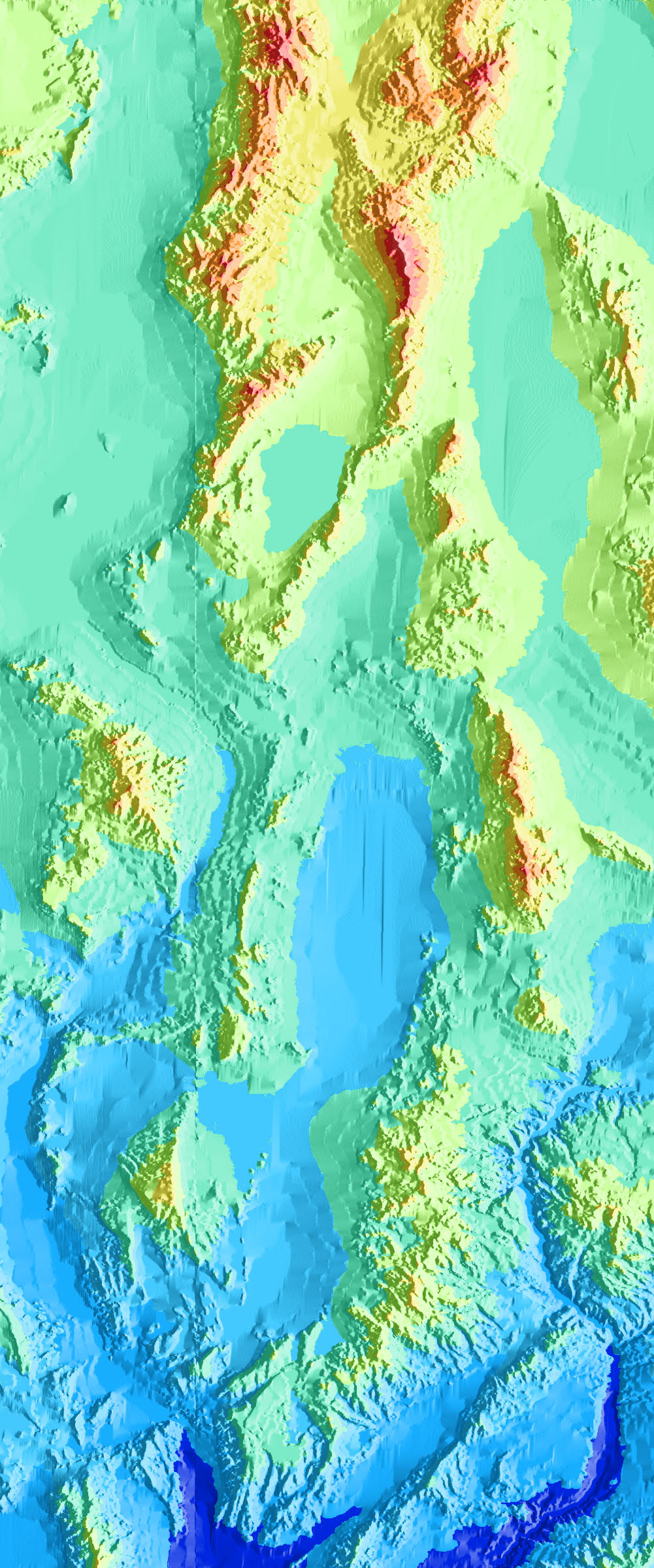
Figure 1. Index map of the study area. 1a) Shaded-relief topography, with labels of the major basins and ranges. Gray lines indicate boundaries of Lincoln, White Pine, and Nye counties
in this and subsequent maps. Dashed lines indicate US Highway 93 and Nevada Route 318. 1b) Generalized geology from Stewart and Carlson (1978). 1c) Index map of Nevada showing study area (hachured).

Shingle Pass Fault 10000 12000
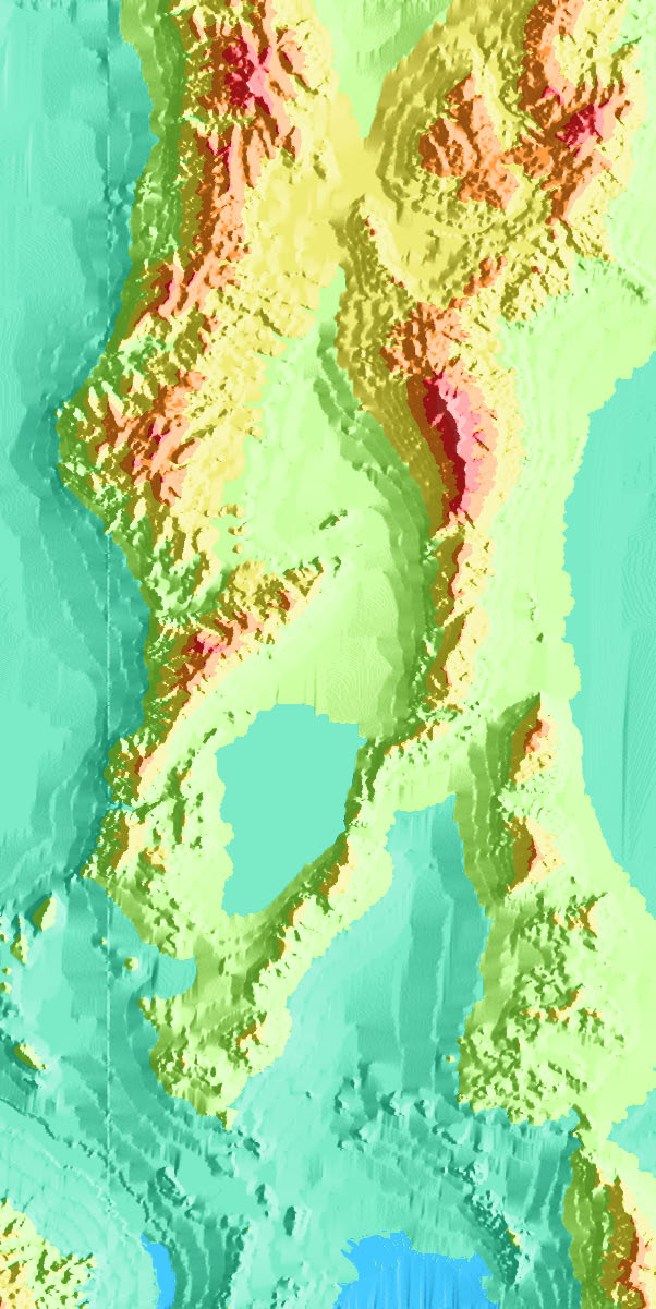
Isostatic gravity anomaly (mGal) Figure 2 . Cave and Muleshoe val ey results. 2a) Shaded -relief topography, with smal black circles indicating gravity stations col ected prior to 2003 and smal
magenta circles indicating gravity stations col ected by the USGS in 2003 and 2004. Larger circles indicate oil and gas wel s; red -fil indicates wel s that pass through the entire al uvial section, and white-fil indicates those that bottom in al uvium. Red triangles indicate MX wel s that pass t hrough the entire al uvial section. Yel ow line indicates the position of the ECN -01 seismic reflection line. 2b) Geology, as in Figure 1b). 2c) Isostatic gravity anomaly map. Red dashed line indicates the outline of the al uvial basins, and thin lines mark the generalized geology of Figure 2b). Pink circles denote the locations of local maxima of the horizontal gradient of the isostatic anomaly field. Only those locations that fal on mapped al uvium are shown, and they are sized according to whether they fal in the lower, middle, or upper thirds of the gradient magnitude distribution. -40.0 -35.0 -30.0 -25.0 -20.0 -15.0 -10.0 -5.0
Basin gravity anomaly (mGal) Figure 2 (continued) . 2d) Basin gravity anomaly derived from the depth-to-basement algorithm described in the text. 2e) Calculated basin depth, based on the basin gravity anomaly (2d).
Symbols of oil and gas and MX wel s are as in (2a), and depths in kilometers to the base of the al uvium are annotated above the symbols. Yel ow line indicates the position of the ECN-01 seismic reflection line.

10000 12000
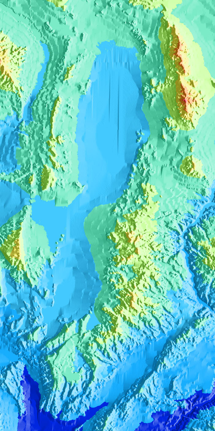
Isostatic gravity anomaly (mGal) Figure 3. Dry Lake and Delamar val ey results. 3a) Shaded-relief topography, with smal black circles indicating gravity stations col ected prior to 2003 and smal magenta circles
indicating gravity stations col ected by the USGS in 2003 and 2004. Larger circles indicate oil and gas wel s; red-fil indicates wel s that pass through the entire al uvial section, and white- fil indicates those that bottom in al uvium. Red triangles indicate MX wel s that pass through the entire al uvial section, and white triangles indicate MX wel s that bottom in al uvium. 3b) Geology, as in Figure 1b). 3c) Isostatic gravity anomaly. Red dashed line indicates the outline of the al uvial basins, and thin lines mark the generalized geology of Figure 3b). Pink circles denote the locations of local maxima of the horizontal gradient of the isostatic anomaly field. Only those locations that fal on mapped al uvium are shown, and they are sized according to whether they fal in the lower, middle, or upper thirds of the gradient magnitude distribution. -40.0 -35.0 -30.0 -25.0 -20.0 -15.0 -10.0 -5.0
Basin gravity anomaly (mGal) Figure 3 (continued) . 3d) Basin gravity anomaly derived from the depth-to-basement algorithm described in the text. 3e) Calculated basin depth, based on the basin gravity anomaly (3d).
Symbols of oil and gas and MX wel s are as in (3a), and depths in kilometers to the base of the al uvium are annotated above the symbols. 3f) Calculated basin depth from Saltus and version (m) 2000
ravit 1800
t depth fr 1200
0 200 400 600 800 1000 1200 1400 1600 1800 2000 2200 2400 2600 2800 3000 3200
Basement depth from well pick (m) Figure 4. Comparison of basement depths from borehole picks (x-axis) vs. those from gravity depth-to-basement analysis (y-axis).
Black circles are wel s where exact basement depth constraints were available; gray circles denote wel s that bottomed in Cenozoic deposits, and hence their depth is a minimum estimate. Because the black points cluster along the 1:1 dashed line, the density-depth relationship is appropriate for this area.

Sidehill Pass &
Muleshoe
Schell Creek R.
Time (sec)ay o-wTw ation (m) -3000
Elev -5000
Longitude (minutes west of 114˚W) Figure 5. Cross section of southern Cave and northern Muleshoe val eys (cf. Figures 2a, 2e). 5a) ECN-01 seismic reflection
section displayed in time. 5b) Results of gravity depth-to-basement inversion with low density basin-fil in yel ow; vertical exaggeration = 1.5. API wel 27-017-05221 is displayed on the section, and its al uvial interval is shown in dark yel ow. Appendix
Table A1. Principal facts for gravity stations collected in 2003 and 2004 in Cave, Dry Lake, and Delamar Valleys. [Datums: latitude and longitude, NAD27; elevations, NGVD29. FAA, free-air anomaly; ITC, inner terrain correction calculated out to 2 km; TTC, total terrain correction; CBA, complete Bouguer anomaly, ISO, isostatic anomaly] Station Latitude
Longitude
Elevation
Observed
(deg min)
(deg min)
33.59 12.90 18.44 -210.30 -7.01 41.24 1.97 5.02 -207.88 59.57 3.15 7.31 -214.71 59.18 2.53 6.31 -213.60 66.26 1.10 5.34 -209.91 75.29 0.63 5.58 -204.09 79.68 1.26 8.12 -203.63 66.31 2.72 10.33 28.60 2.31 5.96 -204.90 43.54 2.11 4.51 -205.76 16.58 2.46 5.20 -203.62 14.59 1.72 4.16 -203.66 10.31 0.97 2.68 -204.23 25.84 1.77 3.64 -201.57 48.99 14.28 20.61 -194.94 1.05 39.61 5.24 8.16 -209.19 39.60 3.37 6.25 -213.69 46.93 1.77 5.46 -213.31 10.84 1.40 3.98 -194.70 1.10 25.31 2.22 3.97 -186.78 5.61 16.01 3.12 4.52 -187.53 4.02 34.39 5.16 7.50 -196.11 57.59 1.39 4.90 -188.42 2.71 49.41 2.52 5.30 -190.93 1.19 47.53 3.31 6.42 -193.25 19.50 0.88 2.08 -195.69 87.98 7.70 21.44 104.96 13.66 37.11 -192.80 2.33 41.24 4.26 7.89 -211.19 30.33 0.80 3.91 -216.05 49.16 3.41 8.00 -215.70 70.95 3.63 9.47 -217.83 64.87 2.75 7.42 -217.95 54.69 1.82 4.80 -218.83 74.15 1.22 6.21 -211.48 70.90 1.17 6.02 -212.23 51.46 0.90 3.02 -218.64 42.82 1.18 3.36 -215.98 109.36 5.61 25.44 -216.83 82.03 5.74 14.44 19.03 0.51 1.58 -202.78 17.32 0.77 2.49 -196.18 1.62 61.12 4.20 9.81 -203.24 68.86 10.91 20.61 -204.03 -5.52 26.24 2.54 4.34 -206.82 82.49 7.79 21.29 90.38 4.39 17.70 101.82 4.77 20.67 -213.12 99.64 6.59 24.18 31.71 0.69 1.98 -200.82 33.68 2.90 4.37 -197.82 27.00 1.54 2.64 -198.09 37.46 2.49 5.26 -209.32 16.76 1.02 1.70 -203.01 41.08 2.62 5.20 -194.65 26.60 0.98 1.82 -190.06 42.72 1.99 4.97 -192.79 44.21 3.59 7.23 -190.77 14.55 0.50 0.99 -199.59 -16.04 0.03 0.50 -199.01 -4.69 -15.37 0.02 0.36 -197.36 -2.95 -22.18 0.01 0.27 -203.11 -8.50 -28.05 0.01 0.23 -208.33 -28.45 0.02 0.21 -209.27 -33.38 0.01 0.21 -213.82 -40.48 0.02 0.26 -220.80 -49.33 0.01 0.36 -229.75 -50.83 0.02 0.49 -232.23 -48.78 0.03 0.65 -232.11 12.24 0.43 2.76 -212.98 42.27 1.90 4.66 -207.38 26.39 2.63 4.79 -207.07 20.84 1.68 3.80 -207.01 22.82 0.08 1.22 -224.57 24.60 0.06 1.28 -224.92 38.49 0.19 2.01 -215.50 40.55 0.47 2.49 -216.33 40.88 0.60 2.46 -215.42 47.55 0.40 2.34 -213.57 38.81 0.31 1.85 -217.80 27.75 0.22 1.49 -224.35 17.53 0.75 1.97 -217.72 15.07 0.18 1.10 -203.81 18.33 0.07 1.00 -206.90 23.70 0.20 1.20 -205.56 24.33 0.41 1.49 -207.58 27.69 0.18 1.43 -209.99 20.00 0.68 2.00 -211.64 17.20 1.11 3.52 -200.34 13.00 1.00 3.37 -197.55 -17.93 0.07 1.25 -208.98 -36.07 0.04 0.91 -221.97 -44.92 0.03 0.77 -229.05 -28.31 0.06 1.04 -216.16 -11.46 0.09 1.42 -205.62 -9.06 16.67 0.04 0.90 -206.66 11.60 0.40 1.60 -227.02 31.88 0.91 2.36 -223.10 19.84 0.72 2.03 -221.85 30.60 1.16 2.55 -218.09 10.15 0.14 1.46 -217.81 13.28 0.19 1.49 -219.64 12.29 0.19 1.84 -210.50 14.14 0.74 1.44 -193.21 2.79 -12.19 0.01 0.51 -217.93 10.79 0.45 0.97 -194.74 0.38 14.63 1.44 1.98 -189.72 4.06 12.31 0.59 1.51 -193.71 19.58 1.08 1.89 -192.79 0.74 17.62 0.80 1.61 -193.05 0.52 15.36 0.59 1.41 -193.50 0.07 14.38 0.38 1.19 -193.94 15.06 0.27 1.06 -192.58 1.01 11.63 0.19 0.96 -195.27 10.22 0.16 0.91 -195.97 -12.71 0.01 0.37 -217.55 -13.32 0.01 0.37 -218.12 -12.07 0.01 0.40 -216.92 11.39 0.67 1.24 -192.88 0.86 13.56 0.99 1.56 -191.11 2.60 15.59 1.32 1.88 -190.22 3.49 17.84 1.35 1.90 -189.83 3.85 30.66 0.26 1.78 -170.01 27.46 0.52 1.99 -168.90 19.16 0.93 2.38 -173.24 14.02 1.34 2.77 -174.21 10.47 1.71 3.15 -174.94 -22.80 0.05 0.74 -190.21 -20.07 0.02 0.65 -179.91 -22.88 0.02 0.55 -180.68 -24.25 0.01 0.51 -179.66 -21.55 0.02 0.43 -177.40 -22.44 0.01 0.50 -178.25 -26.51 0.00 0.43 -182.15 -16.66 0.08 0.58 -180.30 -8.54 -14.19 0.11 0.61 -178.27 -6.01 -11.86 0.34 0.85 -175.14 -2.35 11.32 0.12 0.75 -172.72 3.48 16.50 0.28 1.00 -173.98 3.08 19.40 0.08 0.91 -176.82 0.70 32.26 0.12 1.17 -168.67 9.28 29.63 0.35 1.73 -176.82 1.38 33.13 0.68 2.10 -174.10 4.24 40.38 1.98 4.34 -174.15 4.95 42.80 1.69 4.29 -174.15 5.10 54.11 3.68 7.30 -175.01 4.77 47.58 2.17 5.57 -175.16 4.81 48.35 2.51 5.97 -177.20 3.43 51.67 2.63 6.17 -177.17 3.71 55.22 5.00 8.61 -177.68 3.49 52.05 1.69 4.84 -179.67 1.86 43.89 0.86 3.88 -178.96 2.18 35.74 0.34 2.73 -178.72 2.40 24.46 0.25 2.10 -181.81 13.27 0.19 1.68 -182.67 11.39 0.15 1.46 -176.15 2.92 -13.59 0.06 0.70 -183.16 -5.15 -24.61 0.07 0.59 -187.31 -8.78 -11.80 0.21 1.18 -188.38 -5.44 12.91 0.30 2.04 -188.24 29.53 0.75 2.94 -184.71 43.31 2.16 4.64 -184.34 -23.56 0.02 0.43 -198.99 -14.06 0.04 0.38 -200.09 20.90 0.75 1.49 -189.20 26.02 0.44 1.22 -189.97 14.10 0.06 0.55 -194.36 -20.04 0.08 0.41 -195.35 -9.18 -22.81 0.03 0.28 -197.72 -24.56 0.03 0.27 -198.55 -23.64 0.03 0.27 -196.76 -20.34 0.03 0.26 -192.57 -7.92 -17.98 0.01 0.24 -189.67 -5.29 -28.51 0.03 0.28 -198.34 -32.55 0.02 0.31 -200.42 -32.30 0.01 0.33 -198.84 -17.04 0.03 0.37 -183.62 -1.63 -16.37 0.03 0.37 -182.92 -1.46 -23.55 0.03 0.40 -183.72 -9.21 -18.65 0.04 0.42 -183.79 15.21 0.49 1.59 -169.57 1.02 16.66 1.29 2.32 -171.68 17.36 2.29 3.25 -174.59 21.23 0.50 1.47 -178.35 19.02 0.56 1.44 -178.60 11.97 0.27 0.99 -178.51 18.76 0.36 1.35 -174.87 19.46 0.50 1.52 -173.66 21.47 0.53 1.65 -175.50 18.43 0.38 1.66 -180.23 19.73 0.49 1.93 -182.24 15.83 0.44 1.66 -180.94 11.33 0.19 1.45 -184.32 -26.54 1.14 2.33 -177.08 -5.02 -27.90 0.22 1.17 -185.09 -31.70 0.54 1.81 -183.99 -29.58 0.02 0.37 -195.61 -29.42 0.01 0.36 -195.89 -29.26 0.02 0.38 -195.96 -28.49 0.03 0.39 -195.51 -25.96 0.03 0.41 -194.66 -26.36 0.03 0.40 -194.68 -23.77 0.04 0.46 -194.60 -19.11 0.06 0.56 -192.20 -18.31 2.43 3.76 -161.07 -15.55 1.01 2.21 -164.84 -12.98 0.12 1.02 -170.91 -16.27 0.04 0.73 -172.88 -16.61 0.03 0.60 -172.51 -20.29 0.01 0.50 -175.98 -21.11 0.01 0.47 -176.88 -19.79 0.04 0.50 -175.33 -18.86 0.11 0.55 -174.46 -20.81 0.15 0.56 -177.72 -18.29 0.18 0.64 -177.83 32.82 2.58 4.53 -178.83 34.13 1.07 2.84 -180.70 29.21 0.80 2.36 -177.91 30.40 1.00 2.51 -173.02 43.11 1.40 4.55 -184.36 41.40 3.32 6.80 -182.85 45.17 1.27 4.49 -183.94 46.18 5.15 10.09 44.46 7.87 12.35 40.87 2.20 4.52 -174.72 36.48 1.08 2.83 -171.43 41.24 6.56 10.84 29.06 1.75 3.76 -170.16 20.56 2.42 4.21 -171.89 15.42 2.06 3.95 -178.51 41.82 7.45 13.71 12.20 0.95 2.82 -175.81 14.99 3.58 5.91 -173.61 23.77 4.80 7.73 -169.26 15.44 3.64 5.55 -167.51 -25.52 1.37 1.88 -185.66 -11.47 0.07 0.97 -170.04 -10.97 0.18 1.24 -169.33 21.04 3.61 8.40 -170.02 15.34 5.56 12.06 -17.95 0.37 0.86 -179.81 -20.93 0.40 0.83 -179.82 30.31 7.61 13.01 27.00 2.45 5.42 -176.22 12.00 0.50 2.48 -184.86 10.73 2.96 5.33 -187.51 22.60 1.04 3.59 -179.99 11.90 1.44 3.46 -180.02 -20.14 1.14 1.50 -194.36 -11.51 0.58 0.96 -189.80 38.30 0.88 4.44 -181.68 25.19 2.62 4.31 -176.39 26.61 0.54 1.77 -177.84 36.73 3.67 6.94 -181.61 36.16 4.78 8.41 -182.82 22.13 4.57 6.19 -177.49 -10.22 0.47 0.72 -181.57 0.51 11.42 1.76 2.85 -189.28 26.03 2.73 5.60 -189.31 23.02 2.68 5.07 -188.03 21.75 2.30 4.14 -186.03 32.08 4.40 8.00 -184.89 30.63 3.52 6.38 -183.44 27.05 2.12 3.76 -179.45 36.53 4.42 7.82 -180.96 13.27 0.93 1.80 -176.70 37.54 5.93 9.97 -179.72 1.50 12.96 3.45 5.02 -180.04 0.78 12.09 4.00 5.50 -179.31 1.00 32.74 1.99 3.76 -173.23 4.83 36.11 1.76 3.38 -172.88 4.71 38.70 1.73 3.21 -168.97 7.77 -23.56 0.06 0.75 -194.34 -22.71 0.06 0.75 -192.58 -14.70 0.06 0.94 -178.94 -13.60 0.12 1.05 -180.04 13.69 1.33 3.42 -173.50 23.71 1.28 2.83 -160.16 15.37 0.31 1.53 -158.63 17.46 0.30 1.55 -156.44 21.09 0.46 1.73 -154.77 20.28 0.54 1.82 -157.46 19.90 0.59 1.92 -159.81 21.78 0.57 1.99 -160.63 15.50 0.52 1.87 -164.77 -13.82 0.08 0.91 -177.07 -21.35 0.01 0.59 -180.18 -25.10 0.01 0.50 -182.00 -28.10 0.01 0.43 -183.82 -23.26 0.20 0.60 -178.79 -19.86 0.06 0.48 -177.56 -13.46 0.47 1.06 -178.53 -13.56 0.28 0.93 -180.44 -16.38 0.25 0.85 -181.47 -18.39 0.09 0.65 -181.82 -17.55 0.04 0.56 -179.31 -20.51 0.12 0.60 -180.46 -23.53 0.36 0.77 -179.49 -24.94 0.46 0.87 -180.38 -26.54 0.24 0.66 -182.22 -29.29 0.32 0.75 -185.16 -29.71 0.19 0.62 -186.12 -28.73 0.13 0.56 -186.57 -41.28 0.00 0.43 -198.37 -31.76 0.02 0.45 -189.79 -23.32 0.03 0.51 -183.06 -17.43 0.05 0.62 -180.82 -18.47 0.05 0.58 -180.16 -28.18 0.03 0.51 -187.61 -37.77 0.00 0.44 -196.24 -39.72 0.00 0.45 -198.76 -40.19 0.03 0.54 -200.08 -40.37 0.03 0.54 -200.19 -26.59 0.05 0.85 -190.06 -26.61 0.03 0.83 -190.09 -33.07 0.02 0.71 -194.76 -41.64 0.01 0.55 -200.61 -41.86 0.01 0.44 -198.70 -24.46 0.01 0.50 -181.55 -22.22 0.01 0.70 -183.55 -16.64 0.04 0.82 -177.66 -20.44 0.11 0.59 -180.43 -13.66 0.49 1.08 -178.66 -16.31 0.25 0.85 -181.43 -18.75 0.09 0.65 -182.06 -17.96 0.04 0.56 -179.58 -19.62 0.19 0.74 -181.61 -22.63 0.08 0.64 -184.43 -26.40 0.10 0.67 -186.19 -29.18 0.02 0.54 -190.03 -29.55 0.01 0.49 -191.61 -30.86 0.01 0.44 -194.36 -30.72 0.01 0.45 -194.11 -18.86 0.12 0.58 -188.89 -24.70 0.03 0.44 -192.62 -27.76 0.01 0.42 -194.19 -29.82 0.01 0.42 -194.49 -32.29 0.03 0.51 -196.04 -29.90 0.03 0.58 -196.58 -29.87 0.03 0.49 -193.89 -28.62 0.03 0.50 -194.45 -27.52 0.02 0.44 -192.89 -25.23 0.04 0.57 -195.37 -26.95 0.04 0.49 -195.39 -21.11 0.05 0.56 -194.99 -28.13 0.02 0.38 -195.21 -28.07 0.00 0.32 -194.20 -26.68 0.01 0.30 -193.63 -24.89 0.01 0.28 -192.98 -20.13 0.02 0.28 -190.46 27.75 0.61 1.80 -178.98 -19.68 0.02 0.28 -190.17 -20.12 0.03 0.34 -183.94 -7.16 -42.07 0.00 0.25 -200.67 -23.07 0.01 0.27 -183.73 -6.38 -19.14 0.02 0.35 -182.23 -4.74 -21.43 0.02 0.33 -183.27 -7.64 -17.86 0.04 0.40 -183.63 -8.14 -19.90 0.02 0.28 -190.31 Table A2. Physical property measurements of rock samples collected in 2003 and 2004. Rock type
Grain density
Saturated bulk
Dry bulk density
Porosity
density (g/cm3)
(10-3 SI)
03L002 Carbonate 2.71 03L003 Carbonate 2.67 03L009 Carbonate 2.70 03L010 Sandstone 2.42 03L038 Quartzite 2.64 03L012 Carbonate 2.82 03L013 Carbonate 2.66 03L014 Carbonate 2.68 03L016 Carbonate 2.70 03L017 Carbonate 2.70 03L018 Granite 2.51 2.49 03L021 Carbonate 2.69 03L034 Sandstone 2.62 03L037 Sandstone 2.60 03L023 Carbonate 2.84 03L024 Carbonate 2.84 03L025 Carbonate 2.85 03L026 Carbonate 2.80 03L028 Carbonate 2.64 03L029 Carbonate 2.66 03L030 Carbonate 2.70 03L031 Carbonate 2.68 03L032 Carbonate 2.69 03L033 Carbonate 2.85 03L040 Carbonate 2.70 03L041 Sandstone 2.56 03L043 Carbonate 2.69 03L044 Quartzite 2.64 03L045 Quartzite 2.61 03L046 Quartzite 2.65 03L048 Carbonate 2.70 03L049 Carbonate 2.70 03L050 Carbonate 2.85 03L051 Carbonate 2.81 03L052 Carbonate 2.68 03L053 Carbonate 2.70 03L054 Sandstone 2.60 03L055 Sandstone 2.56 03L057 Carbonate 2.85 03L058 Carbonate 2.68 03L061 Carbonate 2.70 03L062 Carbonate 2.84 03L063 Carbonate 2.86 03L064 Carbonate 2.67 04L015 Carbonate 2.71 04L023 Sandstone 2.47 04L053 Carbonate 2.72 04L062 Carbonate 2.73 04L097 Carbonate 2.74 04L098 Carbonate 2.72 04L100 Sandstone 2.65 04L101 Sandstone 2.64 04L114 Carbonate 2.70 04L120 Carbonate 2.85 04L125 Carbonate 2.76 04L127 Sandstone 2.66 04L128 Carbonate 2.70 04L147 Carbonate 2.69 04L138 Quartzite 2.60 04C028 Carbonate 2.85 04C034 Sandstone 2.63 04C035 Carbonate 2.70 04C036 Carbonate 2.81 04C037 Carbonate 2.75 04C038 Carbonate 2.83 04C067 Carbonate 2.45 04C078 Quartzite 2.57 04C090 Carbonate 2.85 04C091 Carbonate 2.81 04C092 Carbonate 2.39 04C093 Carbonate 2.61 04C094 Carbonate 2.79 04C095 Carbonate 2.67 04C096 Carbonate 2.63 04C097 Carbonate 2.76 04C196 Sandstone 2.63

Source: http://www.forestry.state.nv.us/hearings/past/dry/browseable/exhibits%5CSNWA%5CVolume_7/307_Scheirer_2005.pdf